Theory

Introduction

The Vortex Lattice Method (VLM) is a numerical method used in computational fluid dynamics. It is built on the Potential Flow Theory. Although viscous effects and turbulence cannot be explicitly modelled by VLM, selected flows can be well approximated. VLM allows us to estimate the lift, induced drag, and force distribution of an lifting surface such as an aircraft wing or sail.

Potential flow theory

The potential flow theory treats external flows around bodies as incompressible, inviscid, and irrotational [Tec05]. For a small angle of attack, the fluid flow does not separate abruptly, and the viscous effects are limited to a thin layer next to the body known as boundary layer. In this case, the velocity field can be approximated by a potential function.

The Laplace equation is the qoverning equation in the theory of potential flows:

\[ \nabla^{2} \phi = 0 \]

where \(\phi\) is a potentinal function of the velocity field. It satisfies the conservation of mass and momentum.

Vortex Lattice Method

In VLM, the lifting surface is modelled by a large number of elementary, quadrilateral panels lying either on the actual aircraft surface or on some mean surface, or combination thereof. To satisfy boundary conditions, VLM utilizes following elements to describe each panel:

• source - a point from which fluid issues and flows radially outward such that the continuity equation is satisfied everywhere but at the singularity that exists at the source’s center

• sink - a negative source

• doublet - singularity resulting when a source or a sink of equal strength are made to approach each other such that the product of their strangths and their distance apart remains constant at a preselected finite value in the limit as a distance between them approaches zero

• vortex - an element that generates a circulation, or tangential motion, around its origin

Such singularities are defined by specifying functional variation across the panel and its value is set by determinating strength parameters. Such parameters are known after solving appropriate boundary condition equations. When singularity strengths are determinated, the pressure, velocity can be computed[JJB09].

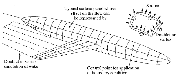
Fig. 1 Representation of an airplane flow field by panel (or singularity) methods. Figure taken from [JJB09] (Fig. 7.22 page 350).

Vortices

The vortex theorems for inviscid incompressible flows has been developed by German scientist Hermann von Helmholtz (1821-1894). The theory is based on the following assumptions [JK01]:

• Flow is inviscid and incompressible

• The strength of vortex filament is constant along its length

• A vortex filament cannot start or end in a fluid (it must form or closed path or extend to infinity)

• The fluid that forms a vortex tube continues to form a vortex tube and the strength of the vortex tube remains constant as the tube moves about.

Vortex element

Vortex element in 2D is presented on figure 2. It is created by placing a rotating cylindrical core in two-dimentional flow field. If the cylinder has a radius \(R\) and a constant angular velocity of \(\omega_y\), then its motion results in a flow with circular streamlines [JK01].

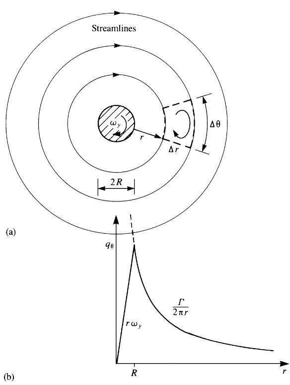
Fig. 2 Two-dimentional flow field around a cylindrical core rotating as a rigid body. Figure taken from [JK01] (Fig. 2.11 page 34).

The tangential velocity, induced by the vortex, can be calculated as:

\[ \overrightarrow{w}_\theta(r) = \frac{\Gamma}{2\pi \cdot r} \]

where \(r\) is the distance from the vortex core.

If a vortex is located in free stream with uniform velocity \(u_\infty\), then the total velocity at the distance \(r\) can be writtes as \(\overrightarrow{u_\infty} + \overrightarrow{w}_\theta(r)\).

Vortex segment

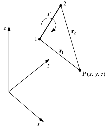
Fig. 3 Vortex segment in three dimensions. Figure taken from [JK01] (Fig. 2.16 page 40).

The velocity induced at point \(P(x,y,z)\) by a straight vortex segement of strength \(\Gamma\) in three dimensions (figure 3) is qiven by equation:

(1)\[ \overrightarrow{w}_{1,2} = \frac{\Gamma}{4\pi}\frac{\overrightarrow{r}_{1} \times \overrightarrow{r}_{2}}{|\overrightarrow{r_1} \times \overrightarrow{r}_{2}|^2} \left(\frac{\overrightarrow{r}_{1}}{||\overrightarrow{r}_{1}||} - \frac{\overrightarrow{r}_{2}}{||\overrightarrow{r}_{2}||}\right) \cdot\overrightarrow{r}_{0}=\overrightarrow{\nu}\,\Gamma \]

where

\[ \overrightarrow{r}_{0} = \overrightarrow{r}_{1} - \overrightarrow{r}_{2} \]

and

\[\begin{gather*} \overrightarrow{r_{0}} = (x_2, y_2, z_2) - (x_1, y_1, z_1) \\ \overrightarrow{r_{1}} = P - (x_1, y_1, z_1)\\ \overrightarrow{r_{2}} = P - (x_2, y_2, z_2) \end{gather*}\]

In case of a semi-infinite vortex line, the point 2 is infinitely far away, thus formula simplifies [PS00]:

(2)\[ \overrightarrow{w}_{1,2} = \frac{\Gamma}{4\pi}\frac{\overrightarrow{u}_{\infty} \times \overrightarrow{r}_{1}}{||\overrightarrow{r}_{1}||(||\overrightarrow{r}_{1}|| - \overrightarrow{u}_{\infty} \cdot \overrightarrow{r}_{1})}=\overrightarrow{\nu}\,\Gamma \]

The Kutta Condition

The Kutta Condition states that at a small angle of attack the flow leaves the sharp trailing edge of an airfoil smoothly and the velocity is finite there [JK01]. Because of this, the normal component of the velocity on both sides of the airfoil must disappear. The flow pattern with circulation consistent with the Kutta Condition is shown in Figure 4.

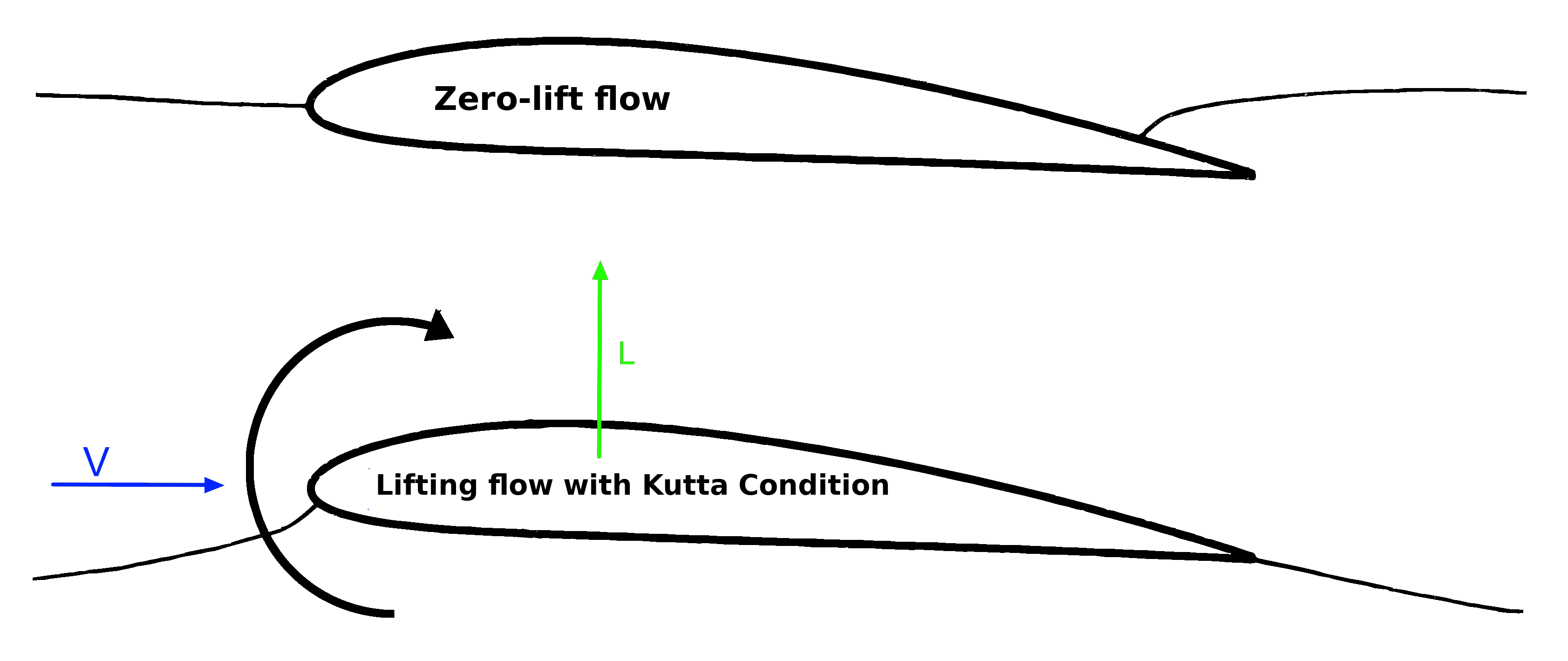
Fig. 4 Flow near cusped trailing edge. Upper figure: zero-lift flow around an airfoil. Lower figure: Upper and lower flows leave the trailing edge smoothly when Kutta condition is applied. Figure taken from [JDA07].

Lifting surface

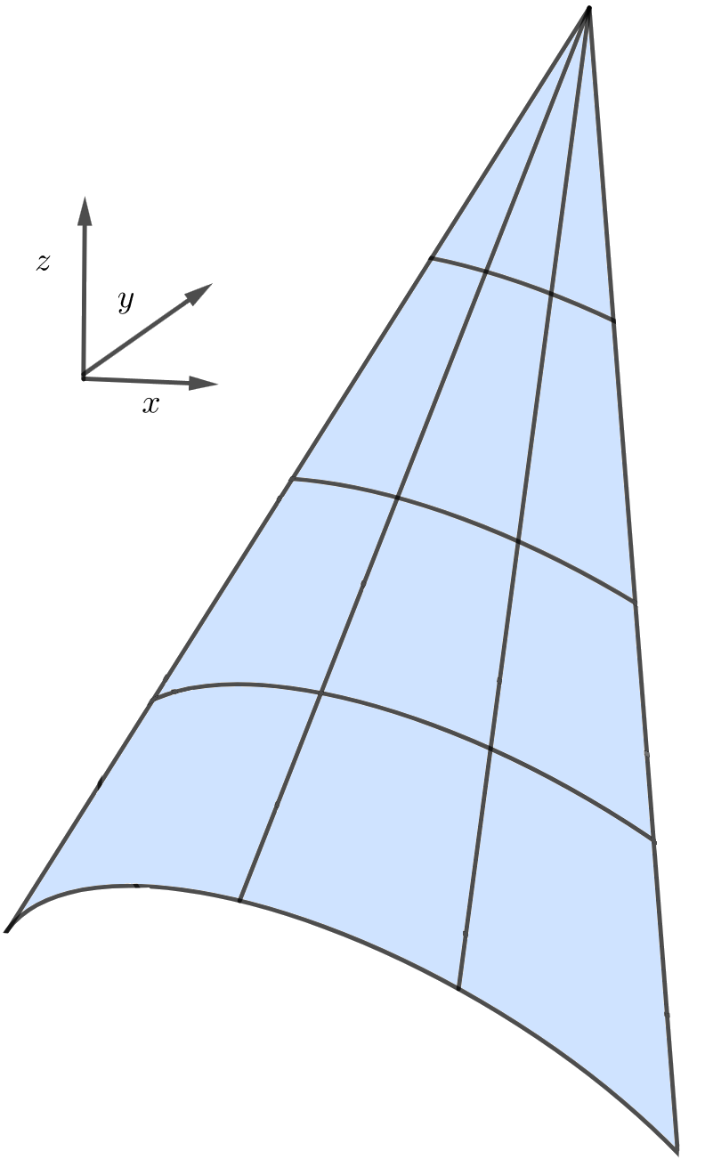
Fig. 5 Sail coordinate system. Figure by author.

The coordinate system (CSYS) (see figure 5) is defined with the x-axis pointing backwards (towards stern), the y-axis in the transverse direction positive to starboard and the z-axis in spanwise direction positive upwards.

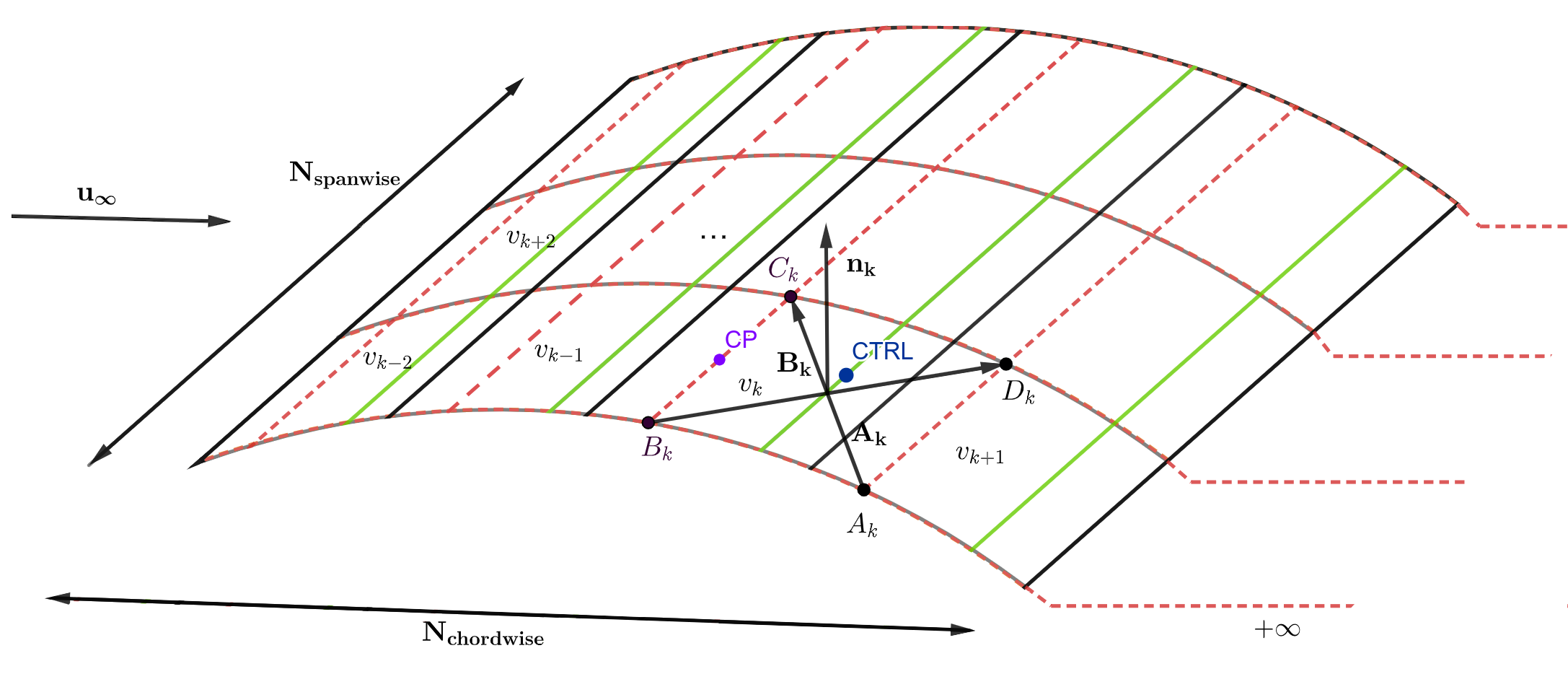
Fig. 6 Nomenclature of the lattice elements. Figure created by author.

The surface of the object is divided into panels ((black rectangles in Figure 6 ). The total amount of them is the product of spanwise and chordwise divisions. The vortex element is associated to segment one of the panel (red rectangles).

There are two types of vortex elements:

• vortex ring

• vortex horseshoe

Vortex ring

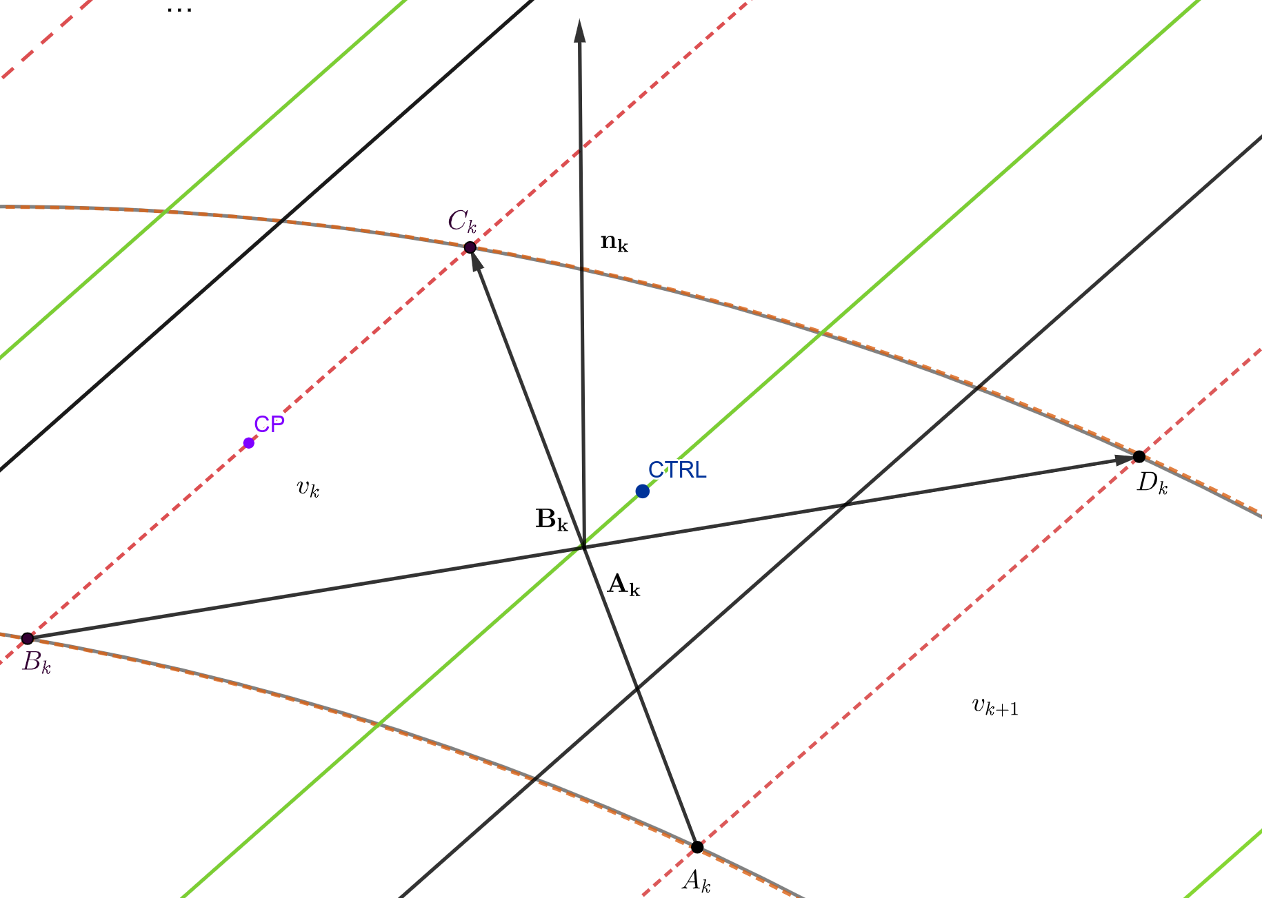
Fig. 7 Nomenclature of the vortex ring. Figure created by author.

Vortex ring (Figure 7) is created by four finite segments according to equation (1).

Horseshoe vortex

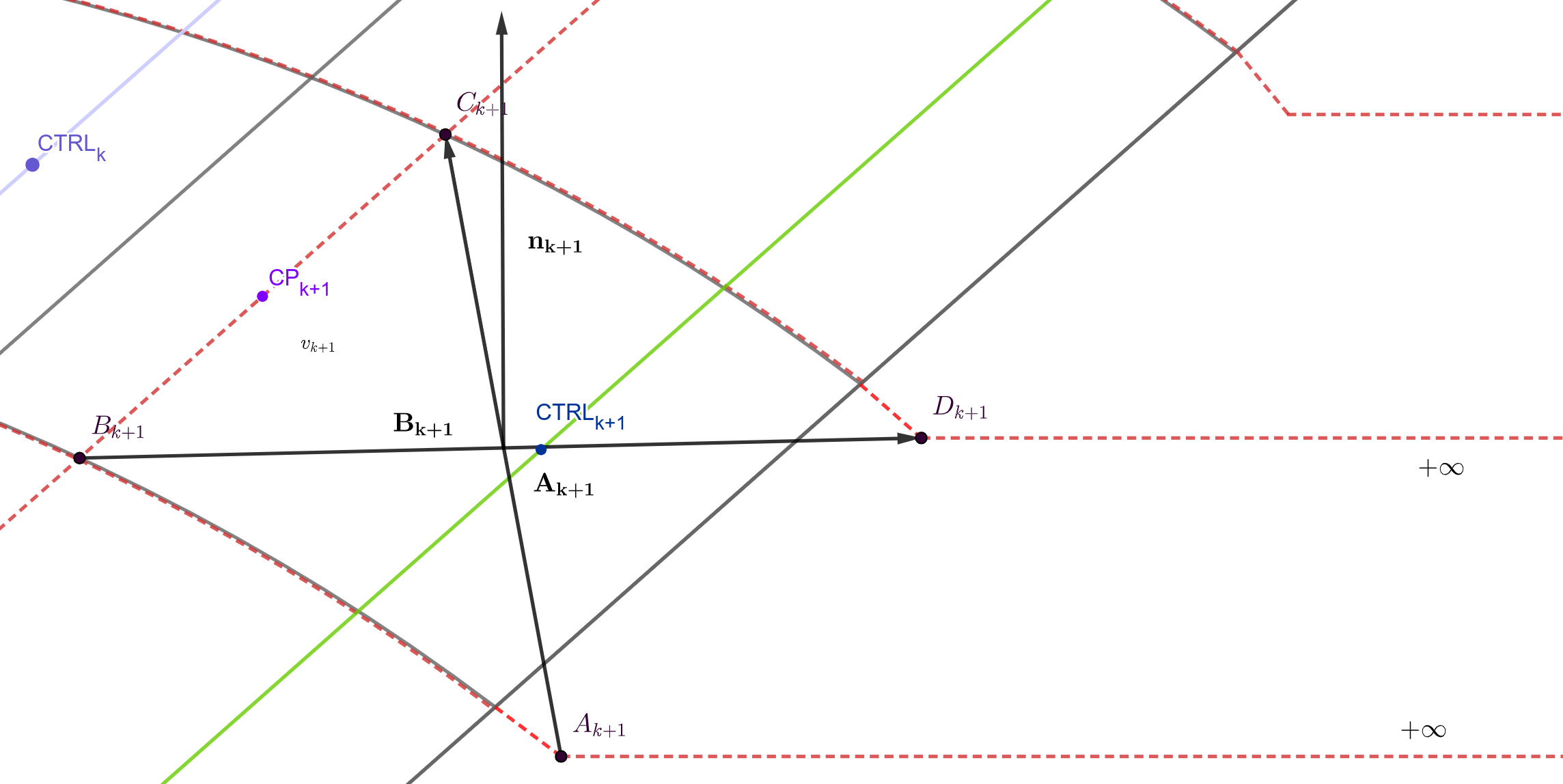
Fig. 8 Nomenclature of the vortex horseshoe. Figure created by author.

Horseshoe vortex is attached to the trailing edge of lifting surface. It consists of three finite segments and two semi-infinite segments following equation (1) and (2) (see Figure 8).

The bound vortex of the wing is considered bound to a “lifting line”. The lifting line theory considers the wing to be a single vortex filament. The tip vortices are the “automatic” consequences of the lifting line and the circulation around a finite wing.

Vortex location

The centre of pressure (CP) is a point to which a resulting aerodynamic force is attached. It is located at the \(1/4\) of a panel chord and at \(1/2\) of the panel span (from the leading edge of the panel). To ensure there is no flow through the surface condition, the control point (CTRL) is defined at \(3/4\) of the chord from the panel leading edge and in the middle of the span.

Each panel has its own index \(k\) (on Figures 6, 7 and 8 symbol \(v_k\) describes the k-th panel). The vortex vertices \(B_k\) and \(C_k\) are placed at \(1/4\) of panel chord, \(A_k\) and \(D_k\) at \(1/4\) of the next panel (\(v_{k+1}\)). The points in the panel opposite the corners define two vectors \(\overrightarrow{A}_{k}\) and \(\overrightarrow{B}_{k}\), and their vector product will point in the direction of \(\overrightarrow{n}_{k}\) (normal vector).

The Boundary Condition

The Boundary Condition requires no flow through the surface of the k-th panel:

\[\begin{split} \overrightarrow{u_k} \cdot \overrightarrow{n_k} = 0 \Leftrightarrow \\ (\overrightarrow{u_{\infty}} + \overrightarrow{w_k}) \cdot \overrightarrow{n_k} = 0 \Leftrightarrow \\ (\overrightarrow{u_{\infty}} + \sum_j \overrightarrow{\nu_{kj}} \Gamma_j) \cdot \overrightarrow{n_k} = 0 \Leftrightarrow \\ \sum_j \overrightarrow{\nu_{kj}} \Gamma_j \cdot \overrightarrow{n_k} = - \overrightarrow{u_{\infty}} \cdot \overrightarrow{n_k} \end{split}\]

Expanding…

\[\begin{split} \underbrace{\overrightarrow{\nu_{11}} \cdot \overrightarrow{n_1}}_{a_{11}} \Gamma_1+ \underbrace{\overrightarrow{\nu_{12}} \cdot \overrightarrow{n_1}}_{a_{12}} \Gamma_2+ ... + \underbrace{\overrightarrow{\nu_{1N}} \cdot \overrightarrow{n_1}}_{a_{1N}} \Gamma_N+ = \underbrace{- \overrightarrow{u_{\infty}} \cdot \overrightarrow{n_1}}_{RHS_1} \\ \underbrace{\overrightarrow{\nu_{21}} \cdot \overrightarrow{n_k}}_{a_{21}} \Gamma_1+ \underbrace{\overrightarrow{\nu_{22}} \cdot \overrightarrow{n_k}}_{a_{22}} \Gamma_2+ ... + \underbrace{\overrightarrow{\nu_{2N}} \cdot \overrightarrow{n_k}}_{a_{2N}} \Gamma_N+ = \underbrace{- \overrightarrow{u_{\infty}} \cdot \overrightarrow{n_k}}_{RHS_2} \end{split}\]

Which leads to a set of linear algebraic equations

(3)\[\begin{gather} \begin{bmatrix} a_{11} & \dots & a_{1m}\\ \vdots & \ddots & \vdots\\ a_{m1} & \dots & a_{mm} \end{bmatrix} \begin{bmatrix} \Gamma_{1} \\ \vdots \\ \Gamma_{m} \end{bmatrix} = \begin{bmatrix} RHS_{1} \\ \vdots \\ RHS_{m} \end{bmatrix} \end{gather}\]

where \(m=n_{spanwise}\cdot\,n_{chordwise}\) and \(a_{kj} = \overrightarrow{\nu_{kj}} n_k\)

The aerodynamic force

Once the system of equations is solved, and \(\boldsymbol{\Gamma}\) is known,

\[ \boldsymbol{\Gamma} = \mathbb{A}^{-1} \boldsymbol{RHS} \]

Then the aerodynamics force can be expressed according to the Kutta-Joukowski theorem,

\[ \overrightarrow{F}_{areo} = \rho \overrightarrow{u}_{\infty} \times \overrightarrow{b} \Gamma \]

Where \(\overrightarrow{b}\) is a span vector.

The aerodynamic force corresponding to the j-th section is:

\[\begin{split} \overrightarrow{F_{j}}=\rho\,\overrightarrow{V}_{app\_wind\_fs\_j} \times \overrightarrow{b_j}\Gamma_{j} = \\ \rho(\overrightarrow{V}_{app\_wind\_infs\_j} + \overrightarrow{w}_{_j}) \times \overrightarrow{b_j}\Gamma_{j} = \\ \rho(\overrightarrow{V}_{app\_wind\_infs\_j} + \sum{\overrightarrow{\nu_{jk}}\Gamma_{k}}) \times \overrightarrow{b_j}\Gamma_{j} \end{split}\]

where \(b_j\) is a vector representing a finite vortex filement going through the centre of pressure of the j-th section, \(\overrightarrow{V}_{app\_wind\_infs\_j}\) is apparent wind velocity for an ‘infinite sail’ (without induced wind velocity) and \(\overrightarrow{V}_{app\_wind\_fs\_j}\) is apparent wind velocity for a ‘finite sail’ (with induced wind velocity).

The pressure is computed as a normal component of a force divided by the area of a panel:

\[ p_k= \frac{\overrightarrow{F}_{k} \, \cdot \overrightarrow{n}_{k}}{S_k} \]

Pressure coefficient at k-th panel follows the formula:

\[ c_p=\frac{p_k}{\frac{1}{2}\, \rho {\left|\left|\overrightarrow{u}_{\infty_k}\right|\right|}^2} \]

Lift \(\overrightarrow{L}\) is the component of this force that is perpendicular to the oncoming flow direction. Total lift coefficient can be calculated from equation:

\[ C_L = \frac{||\overrightarrow{L}||}{\frac{1}{2} \rho_\infty || \overrightarrow{u}_{\infty} ||^2 S } \]

Drag \(\overrightarrow{D}\) is a force that acts opposite to the relative motion of any object moving with respect to a surrounding fluid. The total drag coefficient is defined as:

\[ C_D = \frac{||\overrightarrow{D}||}{\frac{1}{2} \rho_\infty || \overrightarrow{u}_{\infty} ||^2 S } \]

The slope of a lift coefficient:

\[ C_{L,\alpha} = \frac{dC_L}{d\alpha} \]

The slope of a drag coefficient:

\[ C_{D,\alpha} = \frac{dC_D}{d\alpha} \]

where \(S\) is total sail area, \(\rho\) is density of a fluid and \(\alpha\) is angle of attack. \

The section lift coefficient for the chordwise strip is given by the equation (from leading edge to trailing edge):

\[ c_{l,sec} = \frac{\sum_{i} S_i c_{l,i} }{\sum_{i} S_i} \]

The section drag coefficient for the chordwise strip is given by the equation (from leading edge to trailing edge):

\[ c_{d,sec} = \frac{\sum_{i} S_i c_{d,i} }{\sum_{i} S_i} \]

where \(i\) iterates through strip panels, \(S_i\) is a i-th panel area in the strip, \(c_{d,i}\) is drag coefficient per i-th panel in strip and \(c_{l,i}\) is lift coefficient per i-th panel in strip.